

When dealing with sales forecasts that concern fast-moving as well as slow-moving items, we must account for the non-proportional scaling of relative forecast uncertainty with selling rates, which largely determines the achievable level of precision.
Executive summary
- For the same forecast quality, predictions for slow-moving items unavoidably come with a lower absolute but higher relative error than for fast moving ones. Avoid the naïve scaling trap: If your forecast seems to struggle with slow sellers, assess to which extent the increase in relative error when moving towards low velocities is expected.
- There is no hard boundary between ‘slow’ and ‘fast’ movers. Don’t categorize items into different evaluation methodologies, but make sure your evaluation treats all predicted selling rates appropriately.
- Do you encounter many very slow-moving items in your analysis? Challenge that evaluation and make sure your aggregation time scale matches business reality — you don’t take daily business decisions on non-perishable slow-movers.
When abroad, try local, fresh and perishable food specialties
Traveling, though not easy in pandemic times, is an opportunity to learn about other cultures, landscapes and, of course, enjoy great food. Even in today’s connected and globalized world with multi-national retailers that try to instantaneously fulfill every possible wish everywhere on the planet, certain products are simply not offered at all in some places. You might not expect this piece of advice in a blog post on counting statistics, but a direct consequence of our discussion below will be: To culinarily make the most out of your travel abroad, explore the ultra-perishable, fresh specialties. Try fresh fruit in Rio de Janeiro, oven-hot pretzels in Munich and raw seafood in Busan.
Indeed, it’s hard to find traditional Bavarian pretzels in Busan, it’s impossible to buy raw sea cucumber in Rio de Janeiro (as far as we know), and travelers from South America are amused by the restricted choice of fresh fruit in northern European supermarkets. What are the common aspects of these products? They are both perishable and they would be a niche market if sold outside of their original place. Indeed, you get pickled kim chi, exported Oktoberfest beer and cachaça all over the world. But products that retailers would call both ‘ultrafresh’ (very perishable, only good for a day or so) and “slow-selling selling” (likely to not sell on a given day) is never offered, ever, anywhere.
Why is that? Why don’t Brazilian supermarkets try to satisfy the admittedly tiny but certainly existing demand for raw sea cucumber? If 100 sea cucumbers are sold each day in a shop in Busan, and the demand is one per day in Rio de Janeiro, why is the former large demand being addressed by Korean retailers, but the latter is not addressed by Brazilian stores? What is so fundamentally different between a fast-selling perishable item — say, a strawberry in Europe — and a slow-selling selling one — say, a raw sea cucumber in Brazil?
It turns out that retailers don’t offer items of extremely low demand because they cannot predict the actual demand precisely enough to find a profitable sweet spot in the balance between waste and out-of-stock-situations. Generally, a retailer’s business consists in turning consumer demand into actual sales. To know what and how much to have on stock, they need to estimate future demand as well as possible, be it via traditional, human-intuition based or via modern statistics — or even machine-learning-fueled forecasting. Until a few years ago, forecasts in supply chain have been concerned with large quantities on coarse-grained scales, e.g. the total sales of dairy products in a region during a month. Typical numbers that one dealt with were of the order of at least few hundreds, up to many thousands. Today’s computational resources allow forecasting on much more granular level, predictions refer to individual items on a single day in a given location. On that level, the typical numbers that we deal with are not in the 100,000s, but sometimes as small as 5, 1, or 0.1. Can we just transfer the established tooling for forecast assessment from the ‘large-number-world’ into the ‘small-number-world’?
Technically, no problems arise: A computer program written for larger numbers can be run on small numbers. Functionally, however, we need to take care: When moving to the regime of small numbers, statistical idiosyncrasies, which we could safely ignore in the fast-selling regime, become relevant or even dominating. When moving toward slow sellers, we start to experience the limits of forecasting technology: Just like any technology, forecasting has fundamental insuperable bounds. Both the forecast’s precision, the spread of actual demand around the forecasted value, and the forecast accuracy, the absence of bias towards systematically large or small values, cannot consistently overcome certain values, governed by statistical laws. We focus here on lower bound to forecast precision, on the unavoidable level of noise that a forecast of a countable quantity suffers from. This bound turns out to be scale-dependent: The relative uncertainty that we must live with in slow sellers is larger than in fast-sellers. This implies both that our forecast evaluation methodology must be scale-aware, and that you won’t be offered fresh sea cucumber in Rio de Janeiro.
Scale matters
Why do retailers not just scale the stocks on hand with the forecasted demand? If the demand for raw sea cucumber is 1 piece per day instead of 100 per day, just make sure to have 1 piece available instead of 100? If we can reach a 10% error for the fast sellers, we should be able to reach a 10% error on the slow sellers likewise?
This reasoning exemplifies the naïve scaling trap. We encounter naïve scaling in different areas of technology and nature: Isn’t a supermarket just a large store, why do I need to run it differently? Isn’t a country just a large village, why do I need a different kind of administration? Since ants can carry about 50 times their own weight, wouldn’t they be much stronger than us if they had human size? Isn’t an elephant just a large impala, why does it look so different?
We fall into the naïve scaling trap when ignoring that different properties scale differently, as brilliantly described in“Scale: The Universal Laws of Life, Growth, and Death in Organisms, Cities, and Companies” by Geoffrey West, Penguin 2018. A factor of 100 applied to one property of a system, say its weight, does not necessarily imply the same factor for other properties, such as size (quite trivially, as weight scales with the third power of length), or strength (less trivially). Let’s compare an impala to an elephant. Look at the legs of the impala: They are tiny, elegant, fragile. The elephant isn’t only much heavier and larger (it weighs about 100 times the impala, and is about five times longer), it also looks different: Elephants are admittedly elegant in their own way, but clearly their legs are neither fragile nor tiny, but much thicker than the imapala’s, even when accounting for the elephant’s overall larger size. Why is that? Strength and weight scale differently: The factor 100 in weight does not translate into a factor 100 in the elephant’s strength with respect to the impala (even accounting for larger overall proportions), requiring it to have much thicker legs to carry its body. This non-proportional scaling is the fundamental biophysical reason that we don’t encounter mammals that are much larger than elephants — scaling up the elephant by a sizeable factor, the legs of the resulting animal would become thicker than its entire body (huge mammals such as whales have no legs and live in the ocean for a reason). Non-proportional scaling also implies that we don’t have to worry if ants became human-sized: They would not be much stronger than us. Non-proportional scaling makes you run a supermarket differently from a small store, and lets the administration of a country organize it differently from a village. Finally, non-proportional scaling implies that the forecast of a small number comes with higher relative imprecision than the forecast of a large number.
How uncertainty scales
When dealing with predictions, we are especially prone to fall into the naïve scaling trap, because the difference between ‘large’ and ‘small’ are not as obvious as for elephants and impalas: After all, it’s about numbers, which we can easily scale up and down by multiplication and division! An evaluation pipeline ingests numbers of any magnitude, and happily produces evaluation results. Such evaluation setup will technically scale up or down arbitrarily: I can compare a forecast of 1,200,000 against actuals of 1,000,000 using the same tool as for a forecast of 1.2 against an actual of 1. Functionally, however, the 20% error of the large-scale forecast cannot be interpreted in the same way as the 20% error of the latter.
While for elephants, ants and countries, non-proportional scaling is due to the structure of the underlying physical and social networks, non-proportional scaling of forecast uncertainty is implied by the cancellation of positive and negative noise fluctuations under aggregation: Assume you have a daily-level forecast for pretzels with a certain degree of noise. You predict to sell 5 pretzels each day, but sometimes you sell only 3 and need to dispose 2 (don’t even think about eating or selling pretzels that are older than a few hours!), sometimes the demand is 8 (and you have unhappy potential customers); on the long term it averages to 5: Positive and negative fluctuations cancel. The mean absolute error between the forecast and the actual quantifies the typical error, which can be divided by the mean sales of 5 to obtain a relative, percentage value. The smaller this percentage error is, the better. The counts of pretzel demand after one year (365 days) could follow this histogram:
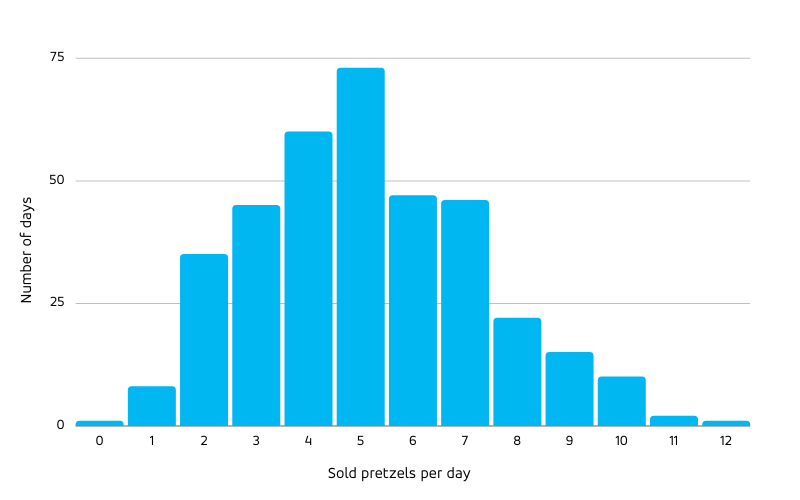
Only on about 70 days did the daily sales exactly match 5, often the sales were a bit off — but the mean sales match 5.
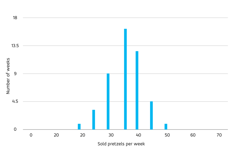
While the decision of the bakery how many pretzels to bake is taken every day, other decisions concern other time scales: Replenishing raw ingredients for the dough doesn’t need to be done daily, but weekly. To evaluate the forecast on weekly level, we aggregate the daily forecast to the entire week, resulting in a prediction of 35 pretzels that can be compared to the total weekly sales. What percentage error do we expect on weekly level? The weekly-level relative error must be smaller than the error on daily level: Days with unusually low sales (4 or less) are balanced out by days with unusually high sales (6 or more). Many individual highly uncertain buying decisions of potential customers add up to a quite certain total sales number. The actual sales in each predicted period of time fluctuate randomly around their predicted value; the more of such fluctuating values we sum up, the more will negative and positive fluctuations cancel. Although the histogram of weekly sales is broader than the above daily one in absolute terms (note that the x-axis changed), it is narrower in relative terms:
The width of the distribution, measured by the standard deviation, increases with the square root of the distribution mean, such that the relative width (the standard deviation divided by the mean) decreases with the inverse of the square root of the mean. In other words: A large forecasted value is the result of many uncertain processes, such that positive and negative fluctuations cancel and give rise to an actual that is relatively close to the forecast, while a small forecast value is only fed by few of such uncertain processes, with fluctuations having a larger chance of surviving and dominating the relative difference between forecast and actual.
This non-proportional scaling of expected forecast error appears, in the first place, for a given product that is forecasted on different time scales: The number of pretzels sold per hour is very uncertain, the number of pretzels per day is more predictable, the number of pretzels per week even more certain. Non-proportional scaling, however, also governs the behavior of different products with different selling rates on a given timescale: the forecast for the number of buns per day (say, about 50) is more precise than the one for the pretzels (about 5), and the latter is much more precise than the one for wedding cakes (about 0.05). Again, this scaling of precision refers to relative errors, while absolute errors increase with selling rates: We might easily sell 5 buns more or less on a given day, whereas the fluctuations of wedding cakes is at most 1 (we typically sell zero, and every now-and-then we sell one).
Just like the strength of an animal does not proportionally scale with its weight, the expected error of a forecast does not proportionally scale with the forecasted value. As a result, elephants don’t look like large impalas and larger forecasted values come with smaller relative error.
Stay tuned to our Blue Yonder blog for Part 2 of this post!