
Summary: In retail forecasting, zero-sales events require special attention when training and applying demand models. It is difficult to find out ex post whether a zero-sales-event truly witnesses vanishing demand on a given day (as in “nobody took that product from the shelf”), or whether the predicted product was simply not available (as in “the product was not even put onto the shelf”). Thankfully, the consistency of the data with the prediction model can be checked by comparing the predicted probability of observing zero to the observed frequency of zero-sales-events. When those do not align well, i.e., one observes zero sales much more or much less often than predicted, one has diagnosed a major but well-defined data problem.
Does Zero Exist, and If So, In How Many Ways?
The number “zero” has evaded the human capability for abstraction for a surprisingly long time. Different ancient cultures treated the “absence of anything at all” in different ways, and historians of science still debate when and how zero as a symbol was invented and became part of the mathematical mainstream. For example, the Roman numerals don’t even contain any symbol for zero, probably because Romans used numbers for accounting, not for arithmetic. Aristotle even rejected the very idea of zero being a number – when you can’t divide by it, what is it good for? In the seventh century AD, the Indian mathematician and astronomer Brahmagupta started to use and analyze a written zero, which then found its way into Chinese and Arabic, and, via the latter, into European culture.
Of course, you know about zero and feel comfortable using it. So let’s fast forward some centuries of mathematical discussions to the prediction of retail demand using artificial intelligence (AI) and machine learning (ML) applications. I argue here that one kind of zero is not enough. At least two different concepts of zero are necessary for the proper description of sales in retail. One must be kept in a training dataset, the other one must be removed.
On the one hand, a product can be available and be offered to the public: The store is open, the cash register and everything else is working – but simply no customer wants to buy it! In that case, the zero sales event reflects the actual lack of demand and the lack of interest of the consumers in that product. Ideally, our demand prediction model is not “surprised” by that zero in the sense that it predicted a not-microscopic but finite probability to observe zero.
Genuine lack of demand leads to a demand-zero, which I’d like to distinguish from the availability-zero. That latter type of zero is induced simply by the unavailability of the product. The customer is not even offered the product, they have no chance to buy it, even if they wanted to (we will never know). I didn’t sell an iPhone for $99 yesterday – but that’s a trivial statement, because I did not even offer any iPhone to anyone. If I had offered it, my moderate price expectation would have induced quite some demand, and probably found a buyer. I did not sell the used stroller that I offered online either – that’s more informative, it’s a demand-zero. While the demand-zero reflects that the item is not particularly popular (to put it mildly), the unavailability-zero has nothing to do with the true demand for an item.
Unavailability can have many different causes: Most importantly, stocks might be depleted – there is then simply nothing left to sell. Therefore, it’s great to have the morning stocks value in a well curated column in our data. Then, we can recur to the methods described in “Why We Expect To Sell Less Than We Predict” blog post. Often, however, such data quality paradise is not what we encounter: Stocks information are unavailable or at least not entirely trustworthy. But even if reliable stocks values were integrated, we can’t be entirely sure that the product is really offered on the shelf – it might be stored in the backroom, the store manager might have decided that it’s too early or too late in the year to offer it.
Unavailability masks genuine demand: To learn about an item’s demand, we need to offer it. I have no idea how much demand a green raincoat with pink sprinkles will induce, unless I put it onto the shelf, put a price tag on it and offer it to customers. If a product is not offered, I can only hypothesize about but not measure demand.
Summarizing, my concepts of zero are these two: The well-behaved demand-zero honestly conveys the (perhaps deceiving) information that the product on the shelf is just not very popular (by the way: anyone out there needs a used stroller?), and the availability-zero, which hides all possible information about the true demand – that demand could have been zero, one, 14 or 2,766. Quite clearly, one needs to include the demand-zeros into the model training, but one would suffer enormously from mistaking an availability-zero for a lack of demand.
How Likely Is a Demand-Zero-Sale Anyway?
In retail, we often deal with the Poisson distribution (read more about it in the “Forecasting Few is Different” Part 1 and Part 2 blog posts). For a Poisson process, the probability to observe 0 decreases exponentially with an increasing mean rate. That is, for a Poisson prediction with a mean rate of 1 (that is, we expect to sell one piece on average), we expect to observe zero in about 37% of the cases – it is, hence, quite likely, and not surprising at all. For a rate of 4, that probability becomes 2% – we expect that to happen every seven weeks or so. For a rate of 10, that probability drops to 0.005%, for a prediction of 20, we are talking about extremely rare events, which would surprise us quite a lot if they occured. The Poisson prediction is, admittedly, an idealization: A realistic demand prediction will be “broader” in the sense that sales values that are far from the mean are more likely in practice than they were predicted by the Poisson distribution. That is, we expect more zero-sales than the numbers above convey.
If we only consider high-selling products, which are bought about 20 or more times per day, any appearing zero can safely be interpreted as availability-zero. Look at the following pattern of sold units in time:
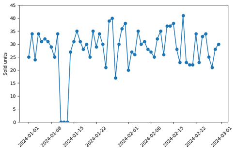
Quite obviously, something exceptional is going on in that mid-January week, when no sales occur for three consecutive days. It’s unlikely that the genuine demand has plummeted so strongly for three days to then shoot back to the initial level. Clearly, we have availability-zeros, which should be removed from the training.
When overall selling rates are not that high, though, it’s not easy to decide whether a given zero is a demand-zero or an availability-zero:
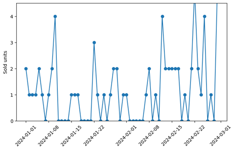
Here, it’s much harder to make the call whether a zero-sale event reflects zero demand or zero availability. Which of those zeros should be kept in the training, which of those should be removed? That question is pivotal for an unbiased training: The mean sales including or excluding the zeros differ substantially.
The low-sales example shows the necessity to include assignment or listing information that tells us, a priori, whether sales can be expected at all on a given day. When the product was not available, the unsurprising and uninformative zero-sales event is an availability-zero. When the product was available, the zero-sales event is a demand-zero, which reflects low demand.
Evaluating Consistency Via the Predicted Zero-Count Probability
Let’s assume we have integrated data, including listing and availability information. We’ve trained a model on the observed demand (including demand-zeros but excluding availability-zeros) and generated predictions. How can we find out whether the information on the type of zeros is correct? For a given sales-event of a slowly moving product (behaving like in the second time series plot), it is impossible to state ex post whether a zero is an availability-zero or a demand-zero. We can, however, make a judgement on a set of many predictions and corresponding observations: We can compare the observed frequency of supposedly demand-zeros to the predicted frequency. For that purpose, we plot the expected rate of zeros against the prediction (which is just an exponentially decreasing curve):
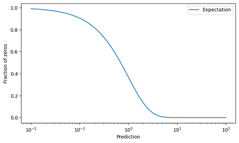
Note the logarithmic x-axis, which spans four orders of magnitude from 0.01 to 100.
Let us now group all predictions and outcomes into buckets characterized by the prediction, e.g., all predictions between 0.8 and 1.2, all between 1.2 and 1.5, and so on. Are you wondering why we group by prediction and not by outcome? The answer is hidden in “You Should Not Have Always Known Better” blog post. For each of these buckets, we plot the observed fraction of zeros into the plot as a circle, with the circle size reflecting the number of observations. We did so here for three different sets of predictions and outcomes, which have different data quality:
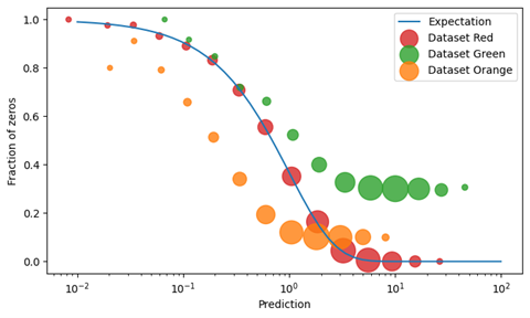
Have a look at the red circles first. For every bucket of predictions, the number of observed zeros in the data matches the predicted fraction of demand-zeros very well. In this case, the data is clean (at least regarding the zeros): Availability-zeros were properly removed, we can trust, on average, that the zeros in the data are truly demand-zeros. We will never know whether the appearing zeros are truly demand-zeros, but there is no evidence to question that assumption.
Now take a look at the green dataset: The observed fraction of zeros is always too large. This points to a systematic problem in the data: When the model predicts 30, one expects no zeros, but observes 30% of zeros in the data. Even if that prediction of 30 were very off and biased, we would never expect such many zeros. Hence, quite a few availability-zeros have incorrectly been treated as genuine demand-zeros. The “plateau” at which the circles converge indicates that there is a constant level of availability-zeros that infect the data. One should check the data and include listing information to make sure that only offered products are included in the sales data. In the individual time series of products, we expect to see artifacts like the one in the figure above.
The orange dataset is an example for the opposite kind of error: For very small predictions, such as 0.1, we expect to see many zeros in the data, but we observe way less. Apparently, some demand-zeros have been incorrectly interpreted as availability-zeros and removed from the dataset. Again, diving into individual products can then help identify the exact cause for this behavior.
In short, a picture like for the red data helps us trust the data, while the green and orange shapes allow us to quickly identify mishandling of demand- and availability-zeros. In our experience, once the zeros-issues are resolved, many other KPIs such as bias also move into the realm of acceptable values.
Make Your Expectation Quantifiable and Explicit, and Compare It to Observation
We did not do any rocket science here, sorry if I mismanaged expectations! We merely asked our model one simple question (“how often do you expect to see a zero outcome for that prediction, on average?”) and we compared the empirical observation to the theoretical answer. Often, a bias in the model is due to an improper handling of zero-sales events. Checking the state of zeros with a plot like the one here should be a standard step in the diagnosis of data problems in demand forecasting projects.
Indeed, the number zero is still often being mistreated in ML applications. The absence of evidence (an availability-zero) should therefore not be interpreted as evidence of absence (a demand-zero). Making this distinction explicit helps us decide on good grounds which datapoint to include in a model training, and which should be removed.