

How to account for finite capacity in demand forecasting training and evaluation
Summary
In retail forecasting, the quantity of interest is the customers’ demand for a certain product, e.g., how many baskets of strawberries are being requested. In practice, one observes a slightly but significantly different quantity, namely the registered sales. Sales reflect the demand, but are constrained by the capacity, that is, by the stocks level: When 20 baskets are in demand, but 12 are available, only 12 are sold, and the 8 customers who were willing to also buy was not fulfilled. The distinction between sales and demand may seem like splitting hairs, but this blog post will show you why mistaking sales for demand leads to biased trainings and flawed model evaluations. You’ll learn how finite stocks impacts sales and how to circumvent the most important pitfalls to confidently tackle real-world situations that involve finite stocks.
Demand and Sales
What is the most precise forecast that you can think of, an always-right demand prediction that you can place any bet on? In many situations, the answer is: Simply forecast “0” all the time! In the view of a demand prediction of zero, not a single item will be ordered, no items will be on shelf, no item will be sold. The zero prediction turns out to be right on spot, perfectly matching the observed zero sales. This absolutely accurate prediction is, obviously, not the forecast that will make your manager happy.
This extreme example illustrates that one should be careful about what to ask for: The goal of a retailer is not to produce a precise forecast, but to operate a sustainable business. The paradox also exposes one fundamental dilemma in demand forecasting: The forecast itself influences the level of stock that is eventually provided, jeopardizing its evaluation. You might argue that this influence exists for good reasons, it is what the forecast was made for! But the stock level sets an upper bound on the number of items that can be sold, which artificially restricts the sales values that can be observed. This leads to a discrepancy between hypothetical demand (“how much is being asked for”) and observed sales (“how much has been sold”). The observed sales are the true demand or the available stocks, depending on what is lower.
In this blog post, I will convince you that there is no way around a rigorous probabilistic treatment of the demand versus sales problem. The distinction between demand and sales, the meticulous treatment of these quantities and of what we exactly predict and observe is key for successful and correct model training and evaluation.
To make things tangible (and savory), we consider a retailer that sells baskets of fresh strawberries. The integer-valued number of sold baskets can then be treated as “pieces.” Unfortunately, these ultra-fresh grocery items go to waste when they are not sold during the day. Therefore, over-ordering, that is, having more on stock than is being asked for, is costly and should be avoided. On the other hand, imagine that you are up for strawberries, but they are already out of stock when you look for them in your local supermarket: You become a frustrated customer, whose willingness to pay has not been scooped up. Hence, under-ordering, having less on stock than is being asked for, is also costly, both in terms of customer satisfaction and lost revenue and profit.
A retailer should order the right number of strawberry baskets to carefully balance out waste and lost sales. Of course, to solve this ordering problem, a precise demand forecast is necessary that truly predicts how many baskets are being asked for, and not how many are being sold (remember the self-fulfilling “0” prophecy above).
How Much Will We Sell?
Let’s dive a bit deeper into demand forecasts and dissect their meaning. A demand forecast tells us how many items will be requested. But what does it mean exactly when “9.7 baskets will be requested”? Clearly, one cannot sell a fractional number of strawberry baskets, the literal interpretation is ridiculous. Still, we accept and intuitively understand the forecast, and interpret it as an assertion about the mean expected number of sold baskets, the number of baskets that we sell on average when the same situation were repeated many times (and stocks are always sufficient, which we will assume for now). Therefore, our forecast implicitly hides some probability distribution, that is, some conception of how likely it is to sell 1, 2, 3, … baskets, since it only states the mean expected sales. What those probabilities are, or how close individual observations (that is, actual sales numbers) are found around that mean of 9.7, is left out.
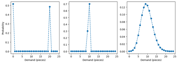
Let’s lift the carpet under which the probability distribution has been hidden to see how it should look like. We’ll use the chart below to illustrate our example. A priori, probability distributions with an expectation value of 9.7 can take very different shapes: Think of a 51.5% probability to encounter zero and a 48.5% probability to find 20, shown in the left panel. This results in a mean of 9.7 – even though one never observes anything close to 9.7, such as 9 or 10, but only extremal values such as 0 or 20. The probability distribution of the middle panel assigns a 70% probability to 10 and a 30% probability to 9; it also bears the expectation value 9.7, but the probability mass is much more concentrated among values close to the mean, which thereby becomes a good estimate for the typical number of sales. The set of distributions with a mean of 9.7 is infinitely large, and most of those distributions will be ill-behaved (or “pathological” as mathematicians like to say). Fortunately, we can assume simple and well-behaved probability distributions, such as the Poisson distribution in the right panel (read the blog post “Forecasting Few is Different” to know why that is a reasonable choice).
Throughout this text, we assume that the forecast produces the mean of a predicted Poisson distribution, and that the demand is truly Poisson-distributed, i.e., that the forecast is correct. Even this idealized scenario will host sufficiently many intricacies to justify a blog post.
How Finite Stocks Censor Information
Let us now welcome finite capacity into the game. Given a demand distribution, we obtain the sales distribution by mapping each possible demand value to the resulting sales value. For all demand values that are below or equate the number of available stocks, demand just translates 1:1 into sales: When there are 12 baskets available, 5 asked-for baskets result in 5 sold, 12 asked-for baskets lead to 12 sold. When demand is larger than the stocks, in other words, when the capacity is not sufficient, the sales are constrained by that stock value: When 13, 25 or 463 baskets are being asked for, only 12 will be sold. When the entire stocks are sold off, we call this a “capacity hit” event. The probability mass associated to the demand of 13, 25, or 463 baskets, however, needs to “go somewhere,” and it is effectively added to the probability that the total stocks are being asked for. The sales probability distributions for a mean demand of 9.7 and different capacities (16, 12, 8) are shown in the next figure.
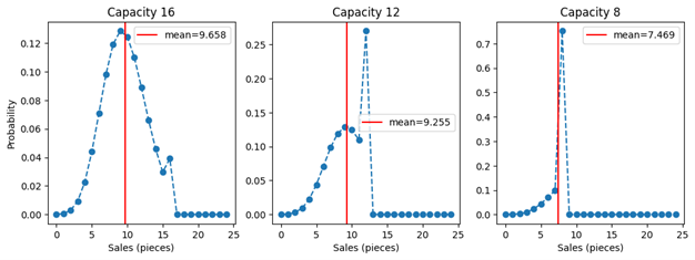
Finite capacity is censoring demand in a way that it removes information: When you put up a capacity of 16 and you observe a capacity hit, that is, 16 sales, you can only infer that the demand was at least 16 – not whether it was 16, 25 or 7,624. The actual demand has some value unknown to you – say, 47 – but you only observe 16. Due to finite capacity, we are truly losing information in an irrevocable way (and not only customer satisfaction). This loss of information both makes it harder to train models under finite capacity and to evaluate them.
The plots also show the expected mean sales as vertical red lines. Perhaps surprisingly, finite capacity has an impact on the expectation value of the sales even when the capacity is still larger than the expected demand. That is, when you predict a demand of 9.7, and you supply 12 items on stock, you sell less than 9.7, on average! You need to stock up more than predicted on average to sell just as much as predicted! This might be confusing: For an individual event, the sales are just the minimum of demand and stocks. But the mean of the sales probability distribution is not necessarily the minimum of the expected demand and of the capacity, as the shape of the probability distribution needs to be accounted for. The reason for this possibly surprising behavior is that the value of the mean predicted demand relies on fluctuations around the mean that cancel out on average. That is, the negative fluctuations (sometimes, less items than 9.7 are being sold) are balanced out by the positive ones (sometimes, more items than 9.7 are being sold). When the capacity is finite, those necessary positive fluctuations are suppressed, and the cancellation of positive and negative fluctuations does not occur anymore. This pushes the mean expected sales to lower values, even when the capacity is larger than the mean expected demand.
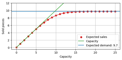
The following plot below shows the expected sales as a function of the capacity, again for an expected demand of 9.7. When the capacity is much larger than the expected demand (say, around 20), events that are affected by the finite capacity are rare. Consequently, the expected number of sales remains unaffected, and close to 9.7. When capacity is small, say, 5, then it is almost inevitable that the capacity is hit, and, on average, a value close to that capacity is sold. Between around 7 and 14, a transition takes place, the capacity has a strong, but not totally determining impact on sales.
Training and Evaluating Models on Censored Demand
Now that we have our workhorse – the probability distribution of sales, aka the capacity-censored demand distribution – under control, let’s understand what we need to be careful about when we train and evaluate models under such circumstances.
We need to distinguish different regimes. If the capacity were hit every day, one would never know the true demand, but only learn a lower bound to it (“we sold 5 pieces, so demand has been at least 5”). This is, fortunately, an unrealistic scenario: When the capacity is hit every day, we deal with lots of unhappy customers and lots of unfulfilled demand – no retailer will sustain such mode of operations for long. If they are forced to do so by supply restrictions, they might consider steering demand by increasing prices.
On the other extreme, when the capacity is never hit, we enjoy the sweet regime to do data science: We read off the true demand every day, we can essentially neglect all discussions about capacity. But the data scientist’s dream is the sustainability officer’s nightmare: A huge amount of waste would be the consequence of such ordering strategy. Given an expected demand of 9.7, we’d need to keep 21 items on stock to run out of stock only once in 1,000 days.
Therefore, one typically encounters a situation in which demand sometimes hits the capacity (and the product is sold out at a given point during a day), and sometimes not (and some stocks remain in the evening). This is reasonable, since a compromise between the competing goals of avoiding waste and avoiding stock-outs is desirable.
We ought to acknowledge that building the best-possible model conflicts with running the best-possible business: Under a sustainable business strategy (when waste is not completely “free”, but being avoided at least to a certain extent), it is unavoidable that products go out of stock sometimes. The best data science, however, is done when stock-outs are guaranteed to never happen, and every sales value directly reflects demand. Since we are doing data science in a business context, we will have to live with the intermediate scenario and occasional stock-outs.
Part 2 of this blog post will share what finite capacity means in practice. It will point out subtle pitfalls that one might inadvertently fall into in order to then share how we typically solve the situation.