

In Part 1 of this blog post, we introduced censored sales probability distributions. Let’s now get our hands dirty and see what finite capacity means in practice. We start by pointing out subtle pitfalls that one might inadvertently fall into in order to then share how we typically solve the situation.
Mistaking sales for demand
Your manager might ask you to just ignore this blog post entirely to obtain both a “first simple model” and a “rough estimate of the model quality.” You might take a deep breath and do so, that is, directly interpret the sales numbers as true demand.
What could possibly happen? A naïve comparison of an unbiased predicted demand against the observed sales will typically produce the verdict “the forecast is biased, it’s overforecasting”: The finite capacity has pushed down the value of the observed sales. The more often one hits the capacity, the more the sales are affected. In practice, what is especially harmful is that the impact of finite capacity will vary considerably between product groups: Fresh products need to go out of stock every now-and-then to avoid waste and capacity is hit every now-and-then. Non-perishables are often replenished in a never-out-of-stock-fashion, and capacity is almost never hit. A comparison between product groups will suffer immensely from the different impact of different capacity / stock-up strategies.
But would we even obtain an unbiased model in the first place? That is unlikely: In training, your model directly learns a biased demand. Of a full demand distribution with a mean of 9.7, the model would only learn the constrained, censored one, which comes with a lower mean value, as can be seen in the figure below:
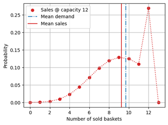
The vicious circle of an under-estimating forecast that leads to a low order, to more stock-outs, to an even more under-estimating forecast is set into perpetually accelerating motion – while the evaluation confirms that “everything is all right” and that the “sales forecast is fine.” In other situations, the capacity constraints during training and evaluation phase might vary due to whatever reason, with pernicious consequences on the interpretation of the observed bias (or lack thereof).
If you read until here, you probably understood that sales and demand are not equivalent, and you will convincingly argue with your manager to go the longer, more precise road.
Selecting days on which demand was not hit
The above pitfall is quite intuitive: Demand and sales are different quantities, and setting them equal when they are not is clearly problematic. The second pitfall that I want you to avoid is a bit more subtle (book a two-hour meeting to explain it to your manager): An idea that typically comes forward in projects is to train or evaluate models on the no-capacity-hit-events alone, i.e., on those days on which the sales have not saturated the capacity. That is, all events for which censoring has taken place (the sales are equal to the stocks) are removed from the training or evaluation, and only sales values that are lower than the capacity are kept. The remaining events are unconstrained ones, which would, that is the hope, make the training and evaluation unbiased.
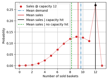
This is, however, not at all the case! By selecting those days on which the capacity was not hit, one naturally selects those negative-fluctuation-events for which the demand happened by chance to be particularly small. That is, one is introducing a selection bias by focusing on those events that are negative outliers. Such a training or evaluation dataset does not reflect the true demand in an unbiased fashion, but produce a negatively biased one. The events for which the capacity was hit are those for which the true demand was, due to random chance, a bit larger than the mean. These events would be necessary to record an unbiased value overall. In the below figure, we see why removing the capacity-hit events can be even worse than training on the entire dataset of sales values (that is, on constrained demand): The mean sales conditioned on not hitting the capacity (green dashed line) are lower than the overall mean sales (red line), because mean sales under capacity hit (black line) contribute to higher values. Remember: What we would like to learn on or what we predicted is the blue dot-dashed mean demand.
Statistically speaking, the days on which one did not go out of stock are not representative for all the days, but they are those on which fewer people came into the supermarket. Maybe strawberries were not fresh, or a promo campaign for mangos made people walk away – in any case, we would be selecting outliers and can’t expect those to be unbiased!
In case you want to go for the reverse strategy, and select those events for which the capacity was hit, you are biasing your dataset even more strongly: The mean sales have then nothing to do at all with the forecast, since they exactly reproduce the capacity setting strategy – the sales then trivially just match the capacity always.
Segregating evaluation data by “capacity was hit” versus “capacity was not hit” also violates one important principle of forecast evaluation: Never split the data by a criterion that was unknown at the moment of the forecast. Such splitting almost always induces a subtle selection bias in the resulting groups. A similar effect is discussed in the blog post “You Should Not Always Have Known Better.”
How to avoid the pitfalls
Regarding training, the conclusion is dire: There is no way around “proper” training using methods such as Tobit regression, which accounts that observing 12 when capacity is 12 only sets a lower bound to the true demand on that day. In other words, we need a regression method that “understands” that 12 sold items means “12 or more items in demand.” Finite capacity truly deletes information – a model that uses capacity-constrained sales as input, even doing so correctly, will always be less precise than a model that uses unconstrained demand.
In model evaluation, one can account for finite capacity explicitly: The expected sales under a given finite capacity can be computed from the censored probability distribution. Again, remember that the expected sales under capacity constraints are not just the smaller value out of “the unconstrained demand forecast” and “the capacity,” but the full constrained probability distribution needs to be considered. One then ends with a comparison like the following:
| Mean uncensored demand prediction | Mean censored sales prediction | Mean actual sales |
| 17.84 | 14.35 | 14.66 |
In this case, one would confirm that the actual sales (after capacity constraints) match the expectation well.
Predicted Capacity Hit Probability and Actual Capacity Hit Frequency
Although comparing the predicted sales under capacity constraints to the actual sales will help establish the bias (or lack thereof) of the forecast and is a good first step in establishing its quality, one often encounters some skepticism along the following lines: “We acknowledge that the forecast is unbiased overall, but we fear that it’s over-forecasting and under-forecasting in an unfortunate way that leads to both more waste and more out-of-stock than necessary.”
In other words, forecasting stakeholders are not only interested in the global lack of bias, but in the lack of bias in every possible demand situation. They don’t want to under-forecast the super-selling days and counter-balance that by over-forecasting the low-selling days. In particular, when capacity is hit, stakeholders want to be sure to hit it only slightly (only few customers leave with their demand unsatisfied); when there is waste, there should not be enormous amounts.
To address this valid fear (you can easily imagine terrible forecasts that are globally unbiased and leave you with lots of waste and unsatisfied customers), I propose to segregate the data by predicted capacity hit probability. That is, given a forecast and a certain stock level that was installed on that day, you compute the predicted probability that the stock is sold out – the predicted capacity hit probability. That capacity hit probability is close to 0 when the stock level is set to a large value with respect to the forecast (e.g., when the stock level is set at the 0.99-quantile of the demand distribution, we are then certain by 99% to not hit the capacity level). The capacity hit probability is close to 1 when the stock level is small, e.g., when it is set at the 0.01- quantile of the demand distribution.
For each prediction, we then have a predicted probability to hit the capacity (e.g., 0.42), and an actual capacity hit (hit or no-hit). Such single hit / no-hit event is merely anecdotical: The mere existence of a few “unlikely” pairs “predicted capacity hit probability = 0.05, but capacity was actually hit” does not mean that the predicted probability is misleading. Only when you have a collection of many probabilistic predictions and associated hit / no-hit events, the predicted probabilities can be verified rigorously. For that, you collect many pairs of capacity hit probabilities (floating-point numbers between 0 and 1) and capacity hits (discrete outcomes, 1 for “is hit” and 0 for “is not hit). Bin these into buckets of predicted capacity hit of around 0, of around 0.10, of around 0.20, etc. For each bucket, you then compute the mean of the predicted and of the actual capacity hit rate. When a capacity hit is predicted to occur in 0.10 of the cases, we expect that in about 10% of those cases the capacity is actually hit.
We call predicted probabilities “calibrated” when we can trust them in the sense that a predicted 0.70 capacity hit occurs in 70% of those cases (learn more about calibration in the blog post “Calibration and Sharpness”). A calibrated forecast allows one to do strategic replenishment decisions: Set the stock level such that you expect to run out of stock in 0.023 of the days – and you truly run out of stock 2.3% of the days. This is risk management: You quantify the risk in a calibrated way, you consciously take those risks that are worth taking.
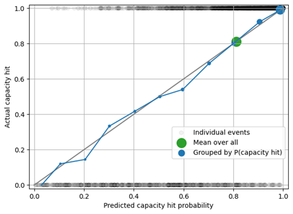
In the figure below, the black circles show individual capacity hit events – capacity was either hit (top of the figure) or not (bottom of the figure). When we group all predictions together, the mean predicted capacity hit rate of 0.82 matches the measured frequency (green circle). When we segregate by capacity hit probability being close to 0, to 0.1, to 0.2, etc., we see that the capacity hit forecast is calibrated: The blue circles are close to the diagonal.
Evaluating predicted against actual capacity hit probabilities and frequencies is not sufficient to ensure a good forecast: When you stock-up 1,000 items, there is no difference in capacity hit behavior between a forecast of 5, 10 or 100 – in all cases, the event ends up in the same bucket “capacity will certainly not be hit.” Therefore, an analysis of bias across predicted sales should complement the capacity hit rate analysis to verify that the forecast is unbiased both across capacity constraints and velocities.
In general, grouping by predicted capacity hit probability or by predicted sales is following the rule “be forward-looking: evaluate what you predict, instead of being backward-looking” to avoid the hindsight bias described in the blog post “You Should Not Always Have Known Better.”
Conclusion: Managing Risk Needs Probabilistic Tools
Point forecasts, which produce a single number as a prediction, are unsuitable to deal with strategic probabilistic questions such as which stock level can assure a stock-out rate below 1%. When you ask a probabilistic question – and all questions about risk are probabilistic – you need probabilistic tools to answer it. You will need to teach your manager at least a basic understanding of “expectation value,” “censoring,” and “distribution.”
Whenever capacity has a real-world impact (and it almost always has), we need to take capacity constraints seriously. We should not try to understand events in hindsight (“the capacity was hit on that day, what was the exact cause?”) but we should look forward and evaluate the calibration of forecasts by segregating them by predicted sales and predicted capacity hit probability.
All the examples in this blog posts were constructed in a sandbox-like environment, assuming a perfect demand forecast that produces a well-behaved distribution. I shielded you from all more complex problems that you’d typically encounter in real-world settings. Still, even in this simple scenario, we see how our intuition is easily fooled. Therefore, it is important to not just follow the very first idea that pops up on how to solve an evaluation problem (“let’s just group by capacity-was-hit versus capacity-was-not-hit”), but to adopt a skeptic perspective and first simulate what the method would do in an ideal setting.