

Part 2: How the Ranked Probability Score reconciles statisticians with practitioners
In part 1, we challenged the usual way to evaluate Mean Absolute Error by just taking the difference between the predicted mean and the observed outcome. We found that it is necessary to use the correct point estimator, the median, to summarize the distribution by a single number, in line with the operational interpretation of Absolute Error. This entails, however, quite a few unpleasant properties of MAE: It’s coarse-grained, discontinuous, and useless for slow-movers.
Clear the stage for the Ranked Probability Score
Clearly, the situation I left you with in the first part of this blog post is not satisfactory: MAE is discontinuous, imprecise, and even useless for slow-movers with predicted means below 0.69. Nevertheless, its reasonable business interpretation — cost is proportional to error — remains attractive. Can we fix it?
Could we just drop the median and use some other summary, like the much more benevolent mean? Unfortunately, pretending that the median/mean distinction is irrelevant does not make it so. Going that route does not resolve our problems, but introduces new ones: The prediction that would win at an incorrectly evaluated MAE would be biased.
What are then our possibilities to improve AE, given that we are tied to the median as a summary? There is one aspect that we can change, namely the order of the two processes “to summarize” and “to compute the error”. Currently, we first summarize (distribution mapped to point estimator), and then compute the error (“point estimator — outcome”). Let’s take a deep breath, and swap the two steps, as illustrated in the plot below (left hand side): Given a predicted distribution (red) and one observed outcome (blue), let’s compute the AE for each predicted outcome (black arrows):
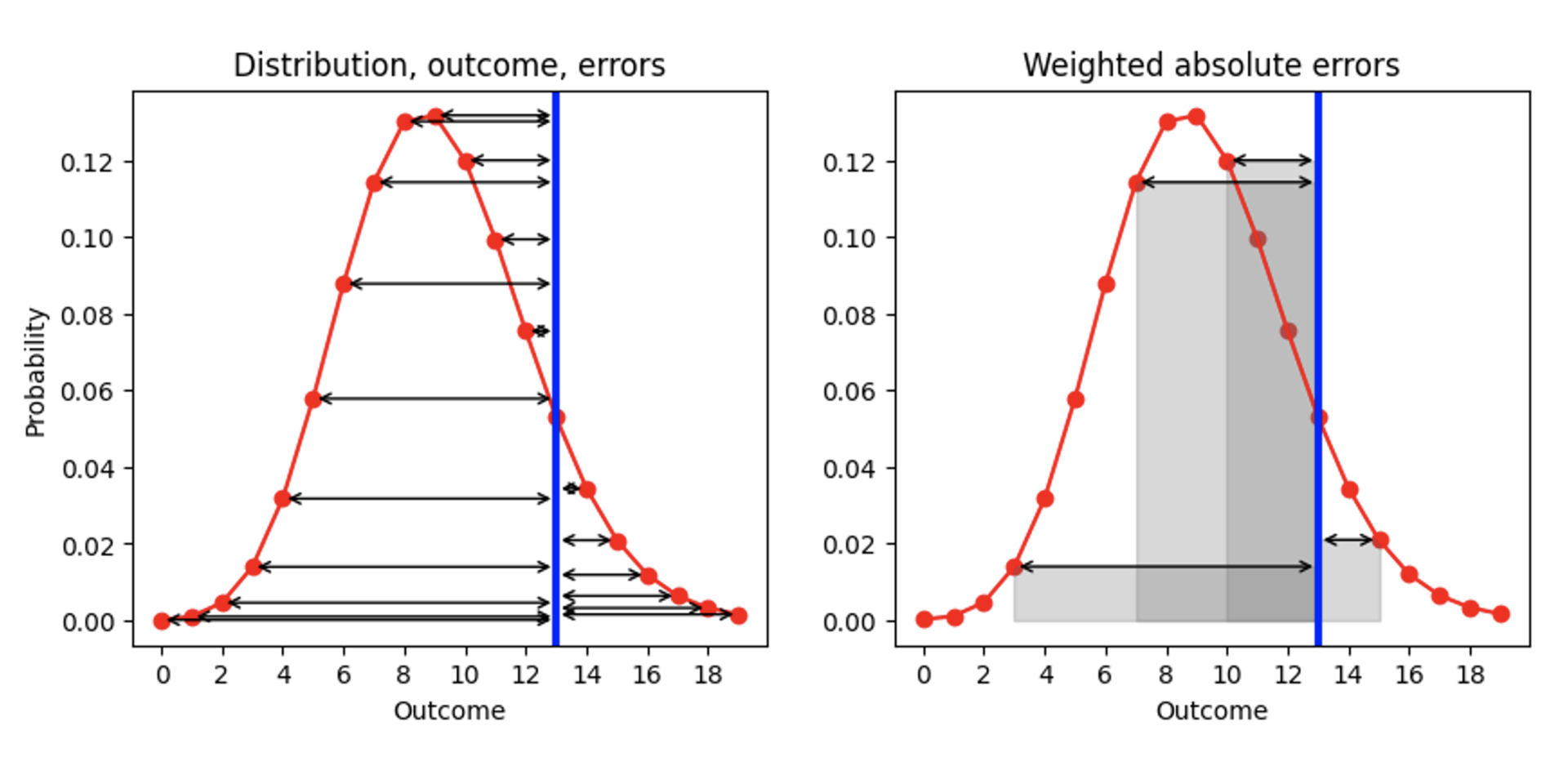
The result is a list of AEs, one for each outcome (including for the prediction that matches the actual outcome, for which AE is 0). Since our goal is to replace AE, a single number, we need to summarize those many AEs. Let’s take the mean of the AEs, with the probability that we had assigned to each outcome as a weight in that mean. Geometrically, we are summing the areas enclosed by the error arrows and the x-axis, as illustrated for a few outcomes in the right plot.
This prescription is a reasonable definition for the distance between a number and a probability distribution: You weight each distance to a possible outcome by the probability assigned to that outcome. As an edge case, if the distribution were 0 everywhere but for one outcome, for which it is 1 (a deterministic forecast that predicts that this outcome will definitely be realized), we recover the traditional AE: The absolute value of the distance between that deterministically predicted outcome and the observation. Our improved AE becomes the traditional AE for deterministic forecasts!
We can express the prescription via this formula:
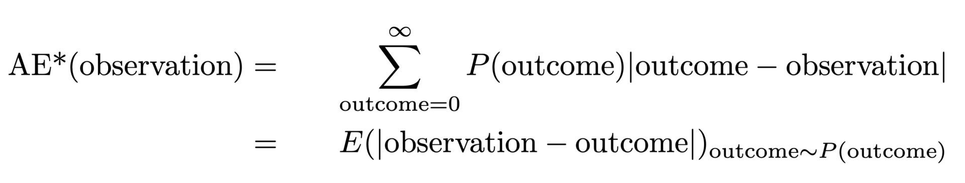
It does look a bit scary, but let’s gently go through it: The AE*, the “corrected AE”, for an observation is the AE for that single observation, but averaged over all possible outcomes (the sum over outcome), with predicted probability P(outcome) as a weight. The second line expresses that this coincides with the expectation value of the absolute distance between observation and outcome, when outcome is distributed according to the probability distribution.
What a ride! We are not there yet, but almost: The AE* is not exactly the Ranked Probability Score, and we still haven’t got a clue where that cumbersome name comes from.
The above-defined AE* has one undesirable property: When the true distribution is a Poisson distribution with a certain mean value, the lowest, best AE* is not achieved when matching that mean value, but for a slightly smaller one. If your forecast wins at AE*, it is probably biased, and underpredicts. The reason is that the absolute width of the distribution increases with the mean value, which favors smaller mean values (yet again an opportunity to advertise the previous blog posts [links to Forecasting Few is Different 1&2]). This problem is solvable: We need to subtract half of the expected width of the distribution to account for that, that is, the expected distance between two random outcomes taken both from the predicted distribution. Finally, this gives us the Ranked Probability Score:

But why is this called Ranked Probability Score (RPS), and why is it so unpopular? The RPS is usually introduced via abstract formulas containing lots of probabilities, step-functions, cumulative probabilities. It is often presented with a purely probability-theoretic interpretation, which makes a lot of sense if you are into probability theory and statistics, but which remains inaccessible to practitioners. It’s truly remarkable that the two formulations — our “improved AE” and the probability-theoretic one — coincide: The ugly duckling (in the eyes of the practitioner) turns out to become a beautiful swan.
How Ranked Probability Score solves the shortcomings of Mean Absolute Error
I argued in the first part of this post that MAE comes with inconvenient properties: It’s coarse-grained, discontinuous, and useless for slow-movers. Does RPS, the “improved MAE”, solve these problems? Indeed, it does!
In the following plot, the RPS (black line) is compared to the AE (blue line), again for an observation of 9 (red dashed line). For predictions that are far from the outcome 9, RPS and AE behave similarly, and RPS just remains slightly below AE. When the predicted mean and the observation coincide at 9, AE hits zero, while RPS is a bit more skeptic: Since RPS is aware of the distribution, it judges that hitting the outcome exactly with the median of the predicted distribution could also be due to chance: Maybe the true selling rate on that day was 7, and we were just a bit lucky that the observed demand was 9. Therefore, RPS never touches 0: No individual outcome unambiguously proves that a probabilistic prediction was correct. When moving away from the outcome 9, AE is strict and immediately penalizes “being off” with the respective cost. RPS is more benevolent here, and does not increase as quickly as AE does, reflecting that “being a bit off” could be due to bad luck, and does not need to be sanctioned immediately. This matches business reality much better: Operations are often planned in a way that slight deviations are tolerable. Everybody wants, but nobody seriously expects a deterministic forecast, and there are safety stocks to account for that. Once deviations are larger, they start to induce real costs.
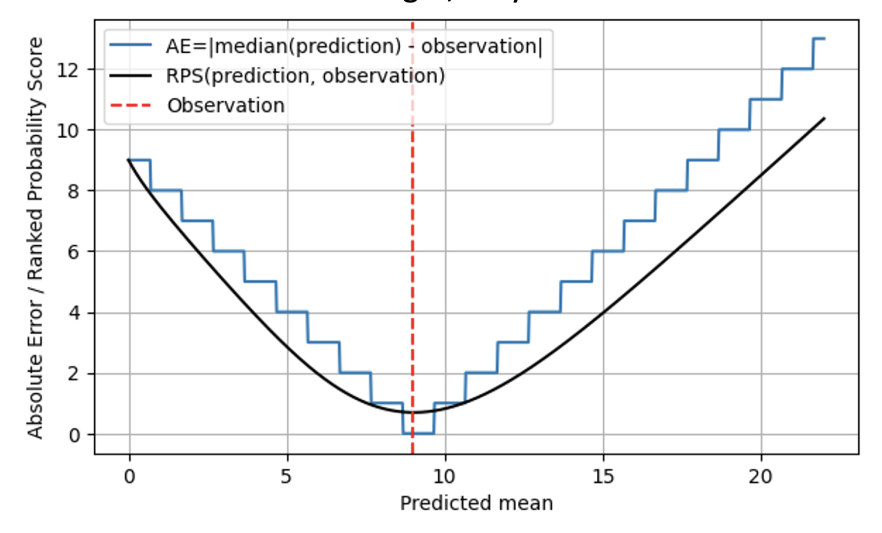
Overall, the Ranked Probability Score does not “jump” between different values, but it is, mathematically speaking, continuous in the predicted mean. For AE, the predictions of 8.7, 9.3 and 9.6 are indistinguishable, for RPS they do become distinguishable: The minimum RPS is reached exactly at a predicted mean of 9.
For slow-movers, RPS helps, but it’s not a magic pill: It will always remain hard to distinguish a product that sells once in 100 days from one that sells once in 200 days, even if you use RPS. Nevertheless, RPS does assume different values even for small different predictions like 0.6, 0.06 and 0.006.
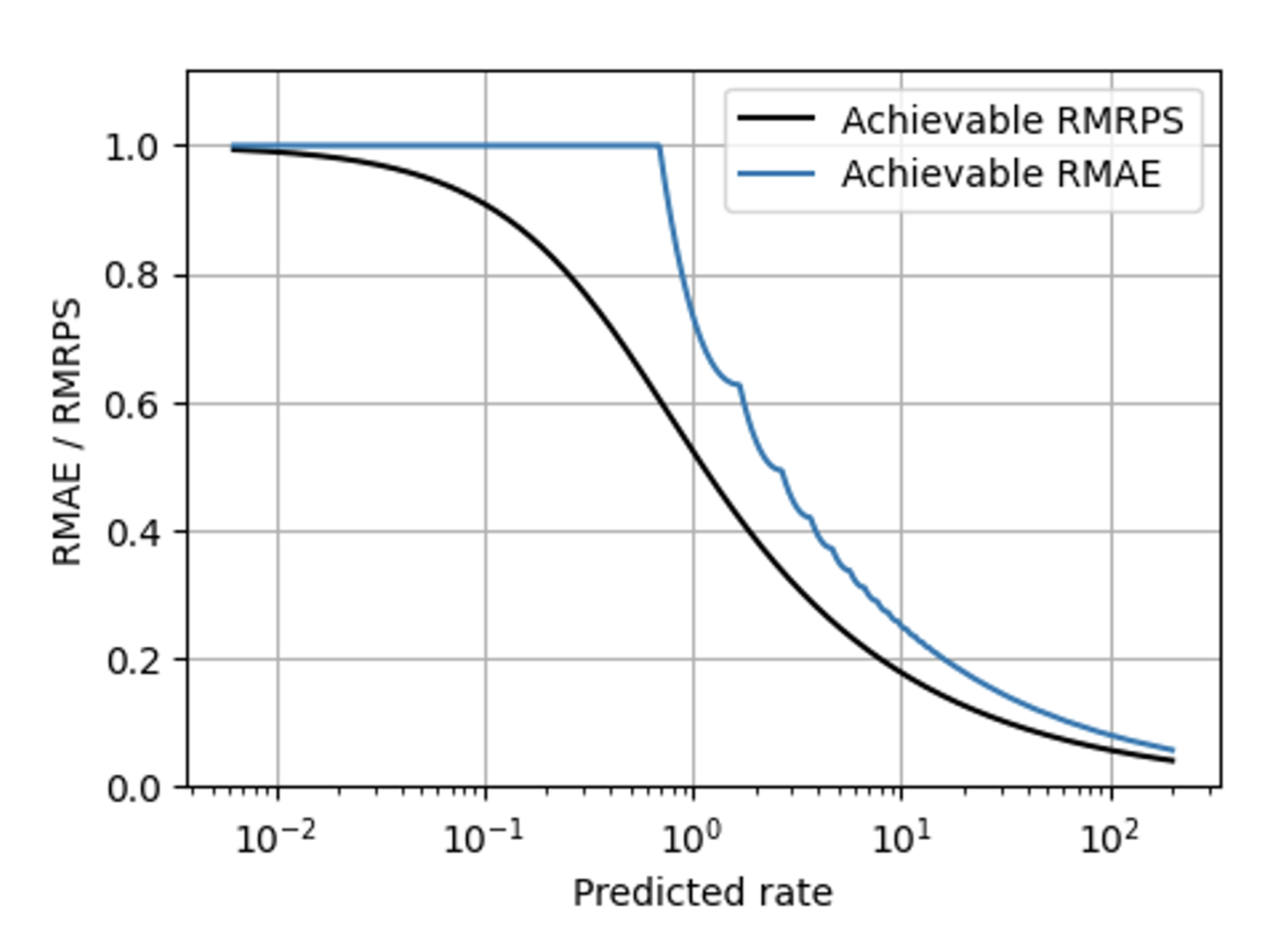
RPS helps with many of MAE’s problems, but there is one challenge which even RPS does not solve: The unavoidable scaling that makes slow- and fast-sellers behave differently. The methods that make metrics scaling-aware (described in parts in this blog [links to Forecasting Few is different 1&2]) can, however, be applied to RPS in the same way they were applied to AE. When compared to the Relative MAE, the Relative Mean RPS (the Mean RPS divided by the mean observation) has a much smoother shape in this plot showing the best achievable value for both metrics:
When should you use MRPS instead of MAE?
Meaningful forecasts are never deterministic and certain, but probabilistic and uncertain, which needs to be accounted for in the evaluation. Saying that humans don’t like uncertainty is a great understatement: Humans hate uncertainty. People are willing to jeopardize a lot of expected utility to achieve perfect certainty (which is, when the risk is fatal, a reasonable thing to do). When business stakeholders are told that a forecast “only” provides a probabilistic prediction, they often want a deterministic one instead, and the forecasters need to disappoint them by refusing to build such. But making unavoidable uncertainty explicit is not a sign of weakness, but of trustworthiness.
Condensing the entire expressive power of a probability distribution, which contains the probability of each thinkable outcome, into a single number is as simplistic, coarse-grained and crude as it seems — although this is what you have to do operationally when you stock up items. From a conceptual perspective, the Ranked Probability Score therefore gives a much better answer to the question “how far is the outcome from the prediction?” than Absolute Error.
Whenever the probabilistic nature of the forecast is irrelevant, the difference between AE and RPS becomes negligible, and AE and RPS can be used interchangeably (the former being simpler to compute than the latter, the latter assuming slightly smaller values). That is, when the width of the probability distribution is much smaller than the typical errors that occur, I, as a forecaster, won’t be able to blame occurring errors to “unavoidable noise against which nothing can be done”. For example, when I forecast certain items to sell 1000 times, and I’m not particularly ambitious and would already be happy when the outcomes are somewhere around 800 to 1200, the difference between using RPS and AE becomes marginal. For simplicity, I should then stick with AE.
Whenever we touch the mid- to slow-moving regime, that is, when we forecast mean values like 0.8, 7.2, or 16.8, it makes a difference whether we condense the distribution into a single number to evaluate AE, or go the slightly more involved path using RPS. When predicting “1”, what we mean to say is that the probability to observe “1” is just about 37%, and so is the probability to observe 0. Neglecting the probabilistic nature of forecasts in the mid- to slow-selling regime is therefore dangerous and misleading. But now you know how to account for the probability distribution: By using the Ranked Probability Score, which I hope you now also see as the beautiful swan of the forecast evaluation wildlife, which achieves to make both statisticians and practitioners happy.