

You Should Not Always Have Known Better: Understand and Avoid the Hindsight Selection Bias in Probabilistic Forecast Evaluation
This blog post on forecast evaluation discusses common pitfalls and challenges that arise when evaluating probabilistic forecasts. Our aim is to equip Blue Yonder’s customers and anyone else interested with the knowledge required to setup and interpret evaluation metrics for reliably judging forecast quality.
The hindsight selection bias arises when probabilistic forecast predictions and observed actuals are not properly grouped when evaluating forecast accuracy across sales frequencies. On the one hand, the hindsight selection bias is an insidious trap that nudges you towards wrong conclusions about the bias of a given probabilistic forecast — in the worst case, letting you choose a worse model over a better one. On the other hand, its resolution and explanation touch statistical foundations such as sample representativity, probabilistic forecasting, conditional probabilities, regression to the mean and Bayes’ rule. Moreover, it makes us reflect on what we intuitively expect from a forecast, and why that is not always reasonable.
Forecasts can concern discrete categories — will there by a thunderstorm tomorrow? — or continuous quantities — what will be the maximum temperature tomorrow? We focus here on a hybrid case: Discrete quantities, which could be, for example, the number of T-shirts that are sold on some day. Such sales number is discrete, it could be 0, 1, 2, 13 or 56; but certainly not -8.5 or 3.4. Our forecast is probabilistic, do not pretend to exactly know how many T-shirts will be sold. A realistic, yet ambitiously narrow (i.e. precise) probability distribution is the Poisson distribution. We therefore assume that our forecast produces the Poisson-rate that we believe drives the actual sales process.
A rather mediocre forecast?
Assume the forecast was issued, the true sales have been collected, and the forecast is evaluated via such table:
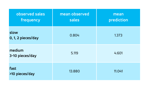
Data is grouped by the observed sales frequency: We bucket all days into groups in which the T-shirt happened to be sold few (0, 1, or 2), intermediate (3 to 10) or many (more than 10) times. At first sight, this table shouts unambiguously “slow-sellers are over-forecasted, fast-sellers are under-forecasted.” The forecast is so obviously deeply flawed, we would immediately jump to fixing it, or wouldn’t we?
In reality, and possibly surprisingly, everything is fine. Yes, slow-sellers are indeed over-forecasted and fast-sellers are under-forecasted, but the forecast behaves just as it should. It is our expectation — that the columns “mean observed sales” and “mean prediction” ought to be the same — that is flawed. We deal with a psychological problem, with our unrealistic expectation, and not with a bad forecast! A probabilistic forecast never promised nor will ever fulfill that for each possible group of outcomes, the mean forecast matches the mean outcome.
Let’s explore why that is the case, how to resolve this conundrum satisfactorily, and how to avoid similar biases.
What do we actually ask for?
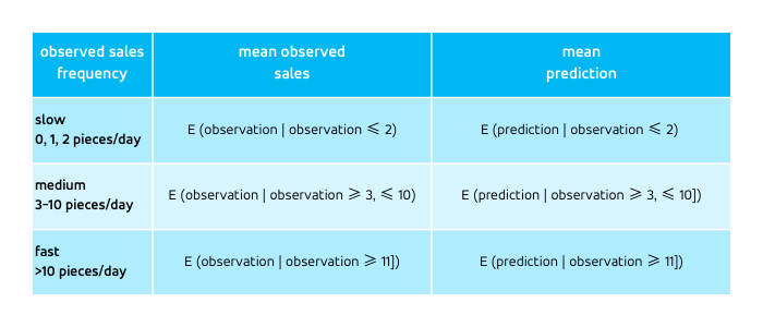
Let us step back and express in words what the table reveals. The data are bucketed using the actually observed sales, that is, we filter, or condition, the predictions and the observations on the observations being in a certain range (slow, mid or fast-sellers). The first row contains all days on which the T-shirt was sold 0, 1 or 2 times, its central column provides us with:

i.e. the mean of the observations in the bucket into which we grouped all observations that are 2, 1 or 0 — definitely a number between 0 and 2, which happens to be 0.804. The right-hand column contains the expected mean prediction for the same bucket of observations,

i.e. for all the observations that are 2 or less, we take the corresponding prediction, and compute the mean over all these predictions.
A priori, there is no reason why the first and the second expressions should take the same value — but we intuitively would like them to: Expecting the mean prediction to equate the mean observation does not seem too much to ask, does it?
Forward-looking forecast, backward-looking hindsight
Consistent with their etymology, forecasts are forward-looking, and provide us with the probabilities to observe future outcomes,

which is the conditional probability to observe an outcome k, given that the predicted rate is x. Since we have a conditional probability, we consider the probability distribution for the observations assuming the prediction assumed the value x. For an unbiased forecast, the expectation value of the observation conditioned on a prediction x, that is, the mean observation under the assumption of a prediction of value x, is:
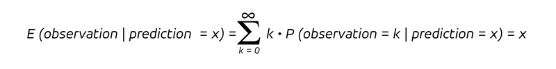
That’s what any unbiased forecast promises: Grouping all predictions of the same value x, the mean of the resulting observations should approach this very value x. While the distribution could assume many different shapes, this property is essential.
Let’s have a look back at the table: What we do in the left column is not grouping/conditioning by prediction, but by outcome. The right-hand column thus asks the backward-looking “what has been our mean prediction, given a certain outcome k” instead of the forward-looking “what will be the mean outcome, given our prediction x.”
To express the backward-looking statement in terms of the forward-looking one, we apply Bayes’ rule,
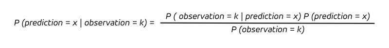
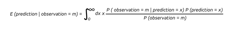
The backward- and forward-looking questions are different, and so are their answers: Other terms appear, P (prediction = x) and P (observation = k), the unconditional probabilities for a prediction and outcome. Consequently, the expectation value of the mean prediction, given a certain outcome, becomes:
Minimalistic example
What value does E (prediction | observation = m) assume? Why would it not just simplify to the observation m?
In the vast majority of cases, it holds E (prediction | observation = m) ≠ m. Let’s see why!
Consider a T-shirt that sells equally well every day, following a Poisson distribution with rate 5. The very same predicted rate, 5, applies for every day. The outcome, however, varies. Clearly, 5 is an overestimate for outcomes 4 and lower, and an underestimate for outcomes 6 and higher. If we group again by outcomes, we encounter:
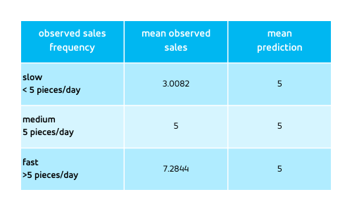
Again, from this table we conclude that the slow-selling days were over-predicted and the fast-selling days were under-predicted, and were indeed. It holds for every observation E (prediction | observation = m) = 5, since the prediction is always 5.
The forecast is still “perfect” — the outcomes behave exactly as predicted, they follow the Poisson distribution with rate 5. The impression of under- and over-forecasting is purely a result of the data selection: By selecting the outcomes above 5, we keep those outcomes that are above the prediction 5 and were under-predicted; by selecting the outcomes below 5, we keep the events below the prediction 5, which were overpredicted. For a probabilistic forecast, it is unavoidable that some outcomes were under-forecasted and some were over-forecasted. By expecting the forecast to be unbiased, we expect the under-forecasting and over-forecasting to balanced for a given prediction m. What we cannot expect is that when we actively select the over-forecasted or under-forecasted observations, that these be not over- or under-forecasted, respectively!
In a realistic situation, we will not deal with a forecast that assumes the very same value for every day, but the prediction itself will vary. Still, selecting “rather large” or “rather small” outcomes amounts to keeping the under- or over-forecasted events in the buckets. Therefore, we have E (prediction | observation = m) ≠ m in general. More precisely, whenever m is so large that selecting it is tantamount to selecting under-forecasted events, we’ll have E (prediction | observation = m) < m; when m is sufficiently small that selecting it is tantamount to selecting over-forecasted events, E (prediction | observation = m) > m.
Deterministic forecasts — you should have known, always!
Why is this puzzling to us? Why do we feel uncomfortable with that discrepancy between mean observation and mean forecast? Our intuition hinges on the equality of prediction and observation that characterizes deterministic forecasts. In the language of probabilities, a deterministic forecast expresses: P (observation = prediction) = 1 and P (observation ≠ prediction) = 0
The forecaster believes that the observation will exactly match her prediction, i.e. predicted and observed values coincide with probability 1 (or 100%), while all other outcomes are deemed impossible. That’s a self-confident, not to say, a bold statement. Expressed via conditional probabilities, we can summarize:

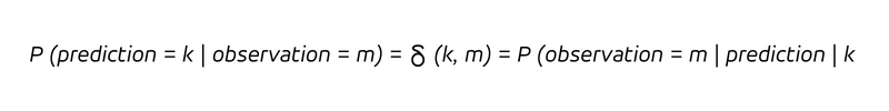
in words, whenever we predict to sell k pieces (the condition after the vertical bar), we will sell k pieces. Since determinism does not only imply that every time we predict k we observe k, but also that every observation k was correctly predicted ex ante to be k, we have:

The determinism makes the distinction between the backward-looking and the forward-looking questions obsolete. With a deterministic forecast, we don’t learn anything new by observing the outcome (we already knew!), and we would not update our belief (which was already correct).
For such a deterministic forecast, for which all appearing probability distributions collapse to a peak of 100% at the one-and-only-possible outcome, no hindsight selection bias occurs — we pretend to have known exactly beforehand, so we should have known — always and under all circumstances. If the measurement says otherwise, your “deterministic” forecast is wrong.
Every serious forecast is probabilistic
Probabilistic forecasts make weaker statements than deterministic ones, and for probabilistic forecasts we must abandon the idea that each outcome m was predicted to be m on average — deterministic forecasts thus seem very attractive. But is it realistic to predict daily T-shirt-sales deterministically? Let’s assume you were able to do so and predict tomorrow’s T-shirt-sales to be 5. That means that you can name five people that will, no matter what happens (accident, illness, thunderstorm, sudden change of mind…) buy a red T-shirt tomorrow. How can we expect to reach such a level of certainty? Were you ever that certain that you would buy a red T-shirt on the next day? Even if five friends promised that they would buy one T-shirt tomorrow under all circumstances — how could you exclude that someone else, within all other potential customers, would buy a T-shirt, too? Apart from certain very idiosyncratic edge-cases (very few customers, stock level is much smaller than true demand), predicting the exact number of sales of an item deterministically is out of question. Uncertainty can only be tamed up to a certain degree, and any realistic forecast is probabilistic.
Evaluation hygiene
There is an alternative way to refute table 1: By setting up the table, we ask a statistical question, namely whether the forecast is biased or not, and into which direction (let’s ignore the question of statistical significance for the moment and assume that every signal we see is statistically significant). Just like any statistical analysis, a forecast analysis can suffer from biases. The way we have selected by the outcomes is a prime example for the selection bias: The events in the group “slow sellers,” “mid sellers,” “fast sellers” are not representative for the entire set of predictions and observations, but we bucketed them into the under- and over-forecasted ones. Also, we used what is called “future information” in the forecast evaluation: the buckets into which we grouped predictions and observations are not yet defined at the moment of the prediction, but they are established ex post. Thus, setting up the table as we did violates basic principles for statistical analyses.
Regression to the mean
The phenomenon that we just encountered — extreme events were not predicted to be as extreme as they turned out to be — directly relates to the “regression to the mean,” a statistical phenomenon for which we don’t even need a forecast: Suppose you observe a time series of sales of a product that exhibits no seasonality or other time-dependent pattern. When, on a given day, the observed sales are larger than the mean sales, we can be quite sure that the next day’s observation will be smaller than today’s, and vice versa. Again, by selecting a very large or very small value, due to the probabilistic nature of the process, we are likely to select a positive or negative random fluctuation, and the sales will eventually “regress to the mean.” Psychologically, we are prone to causally attributing that regression to the mean — a purely statistical phenomenon — to some active intervention.
Resolution: Group by prediction, not by outcome. Remain vigilant against selection biases.
What is the way out of this conundrum? By grouping by outcomes, we are selecting “rather large” or “rather small” values with respect to their forecast — we are not obtaining a representative sample, but a biased one. This selection bias leads to buckets that contain outcomes that are naturally “rather under-forecasted” or “rather over-forecasted,” respectively. We suffer from the hindsight selection bias if we believe that mean prediction and mean observation should be the same within the “slow,” “mid” and “fast” moving items. We must live with and accept the discrepancy between the two columns. Luckily, we can use Bayes theorem to obtain the realistic expectation value. One solution is thus another column in the table that contains the theoretically expected value of the mean prediction per bucket, which can be held against the actual mean prediction in that bucket. That is, we can quantify and theoretically reproduce the hindsight selection bias and see whether the aggregated data matches the theoretical expectation.
A much simpler solution, however, is to ask different questions to the data, namely questions that are aligned with what the forecast promises us. This allows us to directly check whether these promises are fulfilled, or not: Instead of grouping by outcome buckets, we group by prediction buckets, i.e. by predicted slow-, mid- and fast-sellers. Here, we can check whether the forecast’s promise (the mean sales given a certain prediction matches that prediction) is fulfilled. For our example, we obtain this table:
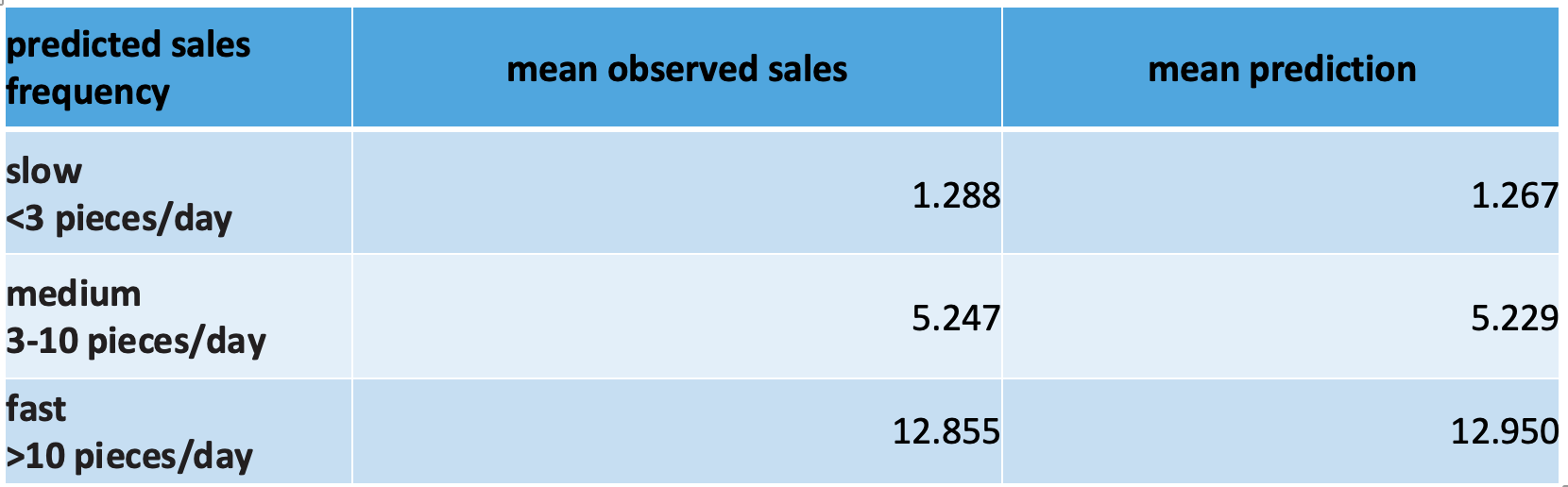
Accounting for the total number of measurements, a test of statistical significance would be negative, i.e., show no significant different between the mean observed sales and the mean prediction. We would conclude that our forecast is not only globally unbiased, but also unbiased per prediction stratum.
In general, you can evaluate a forecast by filtering on any information that is known at prediction time, and the forecast should be unbiased in all tests. However, the filter is not allowed to contain future information such as the random fluctuations that occur in the observations, on which nature decides only in the future of the prediction point in time.
What should you take away if you made it to this point? (1) When you select by outcome, you don’t have a representative sample. (2) Be skeptic towards your own expectations — very reasonably-looking intuitive expectations turn out to be flawed. (3) Make your expectations explicit and test them against well-understood cases.