

This is a two-part story by Malte Tichy about dealing with sales forecasts that concern fast-moving as well as slow-moving items. Find Part 1 here.
How precise can a sales forecast become?
The mechanism of fluctuation cancellation ensures that granular low-scale-forecasts are more imprecise, noisy and uncertain than aggregated, coarse-grained high-scale ones: We are better (in relative terms) at predicting the total number of pretzels for an entire week than for a single day.
So far, we have qualitatively argued for this relation, but can we make any quantitative statement about the level of precision that we can ideally expect, for different predicted selling rates? Thankfully, this is indeed possible, in a universal, industry-independent way. We argued in our previous blog post on hindsight bias in forecast evaluation that deterministic, perfectly certain forecasts are unrealistic: Let’s consider our above forecast of 5 pretzels. On the level of individual customers, a deterministic forecast of 5 translates into 5 customers that will, no matter what, buy a pretzel on the forecasted day. But not only would we assume to know these 5 customers extremely well (maybe better than they know themselves, who hasn’t spontaneously decided to grab or not grab a pretzel?), but we also totally exclude the possibility that any other customer would buy a pretzel. Such degree of certainty is clearly impossible. Allowing some uncertainty, say, 6 customers with a probability of 5/6=83.3% each of buying a pretzel, results in what mathematicians call a binomial distribution in the total number of sold pretzels: The probability to sell 6 pretzels is (5/6)^6, the probability to sell none is (1/6)^6, the probability to sell between one and five contains the respective binomial coefficients. However, knowing 6 customers that will buy with high probability is still unrealistic. Even assuming 10 customers with 50% probability to buy a pretzel each is challenging. We can move on and further increase the number of potential customers while decreasing their probability to buy a pretzel, following the path to the limiting Poisson distribution: In the Poisson limit, we assume an unlimited customer base, in which every customer has an infinitesimally tiny probability to buy, while we have control over the product of the number of customers and the probability to buy: the rate of sale. The Poisson distribution scales consistently: If daily sales follow a Poisson distribution of mean 5, then weekly sales follow a Poisson distribution of mean 35. The Poisson distribution is the “gold standard” for sales forecasting: We assume to know all factors that influence the sales of a given product, but have no access to individual-customer-data that would allow us to make stronger statements on the buying behavior of individual customers. When your forecast precision is as good as expected from the Poisson distribution, you have typically reached the limit of what is possible at all.
A Poisson distribution only ingests a single parameter, the rate of sale; the distribution width, the spread of likely outcomes around the mean, is fully determined by its functional form, which reflects self-consistency. That is, the achievable degree of precision only depends on the predicted selling rate within the considered time interval: The sales of 5 predicted pretzels per day follow the same distribution as the sales of 5 predicted birthday cakes per week, 5 predicted buns per hour or 5 predicted wedding cakes per quarter. In other words: The best-case-achievable relative error is fully and uniquely determined by the forecasted value itself!
Why ultrafresh slow sellers cannot be offered sustainably
With this insight on error scaling in mind, let’s return to the question why fresh sea cucumber is not offered everywhere in the world: We show the expected distribution of sales per day for a perfect Poisson forecast of one sea cucumber per day:
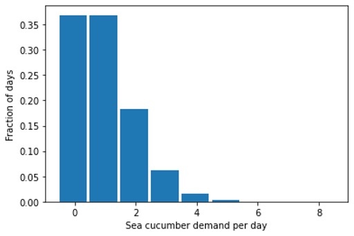
We will experience 37% of days without any demand, 37% of the days will see one seafood-aficionado wanting to buy one raw sea cucumber, and in 26% of the days, we will see a demand of two or even more. How many sea cucumbers shall we keep on stock, given that we must throw them away at the end of the day if nobody buys them? If we have one piece on stock, we’ll have to throw it away in 37% of the days, while in 26% of the days, we’d have unhappy customers that won’t be able to buy the sea cucumber that they intended to. With two pieces on stock, we need to throw away at least one piece after 74% of the days — what a waste, given that sea cucumbers are protected in many places! Clearly, a business model that aims at fulfilling the tiny demand of raw sea cucumber is not viable, and could only be sustained if the margin were extremely large: The people buying the raw sea cucumber need to subsidize all the days on which no sea cucumber is sold — and these people won’t even be sure to get one if they want one! Under mild assumptions on the margin and the costs of disposal, the right amount of stock for an ultra-fresh super-slow seller is: zero.
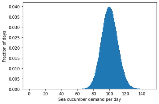
Again, this is all due to non-proportional scaling: The expected distribution of sales for a forecast of 100 fresh sea cucumbers per day is not just an inflated version of the above one for 1 sea cucumber per day, but it has a different shape – just like an elephant does not look like a large impala:
Bad news for anyone who is hoping for getting pretzels in Busan or a wider variety of fruit in northern Europe! There is, however, hope: When demand overcomes a certain threshold because a perishable dish becomes à la mode, that novel food can establish itself in new places — you get good sushi almost everywhere on the planet.
Summarizing, due to non-proportional scaling of forecasting error, the occurring over-stocks and under-stocks of a product — even assuming a perfect forecast – increases disproportionally when the sales rate decreases. Consequently, only above a certain sales rate per shelf life can offering a certain perishable food be sustained at all.
Assessing forecast error
We have now understood why we can’t expect to find foreign fresh delicacies at home, let us now derive some lessons for data scientists and business users in charge of judging forecast quality: For high predicted selling rates, the random fluctuations that drive the true sales value up or down with respect to the forecasted mean cannot be used as an excuse for any substantial deviation, and we can attribute such deviation to an actual error or problem in the forecast. The statistical idiosyncrasies that we discussed above do not matter. If a total demand of 1’000’000 was predicted and total sales amount to 800’000, this 20% error is not due to unavoidable fluctuations, but due to a biased forecast.
For small forecasted numbers, we can’t unambiguously attribute observed deviations to a bad forecast anymore: Given a forecast of one, the observation 0 (which is 100% off) is quite likely to occur (with probability 37%), and so is the observation 2 (which is also 100% off). Judging whether a forecast is good or bad becomes much harder, because the natural baseline, the unavoidable noise, is predominant.
Shall we then divide our forecasts into “fast sellers”, for which we attribute observed deviations to forecast error, and “slow-sellers”, for which we are more benevolent? We recommend against that: What about the intermediate case, a prediction, of, say 15? Where is the boundary between “slow” and “fast”? If a product becomes slightly more popular, what if it crosses that boundary, and its forecast quality judgement takes a sudden jump? There is a continuous transition between “fast” and “slow” that exhibits no natural boundary, as we can see in this plot of the expected relative error of a forecast as a function of the forecasted value (note the logarithmic scale on the abscissa and that we compute the expected error using the optimal point estimator, which is not the mean but the median of the Poisson distribution):
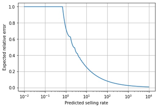
Due to this continuous transition, we recommend a stratified evaluation by predicted rate, which means grouping forecasts into bins of similar forecasted value and evaluating error metrics separately for each bin. Our previous blog post on the hindsight bias explains why this binning should be done by forecasted value and not by observed sales, even though the latter feels more natural than the former. For each of these bins, we judge whether forecast precision is in line with the theoretical expectation (shown in the above plot), or deviates substantially. Our expectations of a forecast should depend on the predicted rate: For extremely small values (smaller than 0.69), most observed actual sales are 0, and we are essentially “always off completely” with an error of 100% — unavoidably. For a predicted sales rate of 10, we will have to live with a frightening relative error of 25% – in the best case! When we forecast 100=10^2, we still expect a relative error of about 8%, for a rate of 1’000=10^3, the error drops to 2.5%. Asking, e.g., for a 10% error threshold across all selling rates is, therefore, counter-productive: The vast majority of slow sellers will violate that threshold and bind resources to find out why “the forecast is off”, while some improvement could still be possible for fast-sellers that obey the threshold and therefore get no attention.
In practice, the deviation from the ideal line that we have drawn above will depend on the forecast horizon (is it for tomorrow or for next year?) and on the industry (are we predicting a well-known non-seasonal grocery item, or an unconventional exquisite dress on the thin edge between fashionable and tasteless?). Nevertheless, accounting for the universal non-proportional scaling of forecasting error is the most important aspect that your forecast evaluation methodology should fulfill!
Conclusions: Avoid the naïve scaling trap, accept and strategically deal with slow-seller noise
Apart putting visits to local restaurants onto your next vacation’s must-do-list, what conclusions should you take out of this blog post?
Make sure that the temporal aggregation scale that you set in your evaluation matches the business decision time scale: Since strawberries and sea cucumbers only last for a day, they are planned for a day and an evaluation on daily level is appropriate. You can’t compensate today’s strawberry demand with yesterday’s overstocks or vice-versa. For items that last longer, the scale on which an error in a business decision really materializes is certainly not a day: If a shirt was not bought on Monday, maybe it will be on Tuesday, or two weeks later — not important for the stock of shirts that is ordered every month. If you encounter many items with small forecasted numbers (<5) in your evaluation, double-check that the latter is really the relevant one, on which a buying, replenishing or other decision is taken.
Don’t set constant targets for forecast precision across your entire product portfolio, neither in absolute nor in relative terms: Your fast-sellers will easily reach low relative errors, your slow sellers will seemingly struggle. Instead, divide your predictions into buckets of similar forecast value, and judge each bucket separately. Set a realistic, sales-rate-dependent target.
For slow-sellers, it is imperative to be aware of the probabilistic nature of forecasts, and strategically account for the large unavoidable noise, be it via safety-stocks-heuristics in the case of non-perishable items, or by produce-upon-order strategies, e.g. for wedding cakes.
Although the unavoidability of forecasting error in slow sellers might be irritating, it is encouraging that the limits of forecasting technology can be established quantitatively in a rigorous way, such that we can account for them strategically in our business decisions.