

The deceiving surprises that Mean Absolute Error hides from us
Executive summary
Mean Absolute Error is the first choice for practitioners when it comes to evaluate their model, owing to its simple definition and its intuitive business relevance. The evaluation metric Ranked Probability Score, by contrast, is not really a charming function at first sight: Its deterrent name fits well with its cumbersome formal definition, which explains that almost no supply chain practitioner knows it, let alone uses it. But they are missing out! The Ranked Probability Score is the natural extension of Mean Absolute Error to the realm of probabilistic forecasts, i.e. to forecasts that “know” about their own uncertainty. It comes with an intuitive interpretation and solves several of Mean Absolute Error’s serious problems. The Ranked Probability Score reflects business even better than does Mean Absolute Error, and it accounts for statistical uncertainty, thereby reconciling ivory tower statistical theory with everyday practice.
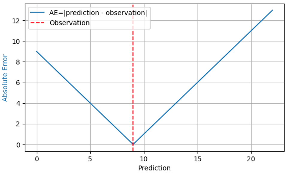
A plausible business standard: Mean Absolute Error “Which metric shall we use to evaluate the demand forecasting model?” That question is typically answered by “Mean Absolute Error,” and on quite solid grounds. Absolute Error (AE) often reasonably reflects the cost of a forecast “being off:” When I forecast 8 baskets of strawberries to be sold, stock up 8 baskets, but the real demand is 9, I have an AE of 1, and 1 unhappy customer turns to competition. When my forecast is 11 baskets for the same demand of 9, the AE is 2, and I have 2 baskets of strawberries to dispose. For that observed outcome 9, the AE is shown by the blue line in the following plot as a function of the prediction:
Since the financial impact of a forecasting error is typically proportional to the forecast error itself, the mean of AE across many predictions and outcomes, Mean Absolute Error (MAE), reflects business cost, at least under the assumption that one piece of overstock has the same financial impact as one piece of understock. Mean Squared Error (MSE) would rate that “being off by one” becomes more costly, the larger the error already is – quite unrealistic in business. Mean Absolute Percentage Error (MAPE), the mean of the normalized AE, Mean (AE/observed outcome), suffers from serious unexpected pitfalls (as described in this previous blog post), and can be safely dismissed for demand forecasting.
Therefore, practitioners are well advised to use MAE or its normalized variant Relative MAE, RMAE = MAE / Mean(outcome), as a first simple choice to evaluate their models. The typical values of MAE and RMAE are, however, scale-dependent: The forecast for bottles of milk (fast-sellers) will naturally come with larger MAE and lower RMAE than the forecast for some special batteries (slow-sellers). That’s admittedly not easy to see, which is why the blog contribution dedicated to that issue did not even fit a single post but was split into Forecasting Few Is Different part 1 and part 2.
With MAE being simple, well-known and relevant, why write or read a blog post on an alternative? Well, blindly trusting an evaluation metric is certainly one of the most data-un-scientific things to do. Let’s do a thorough deep dive of MAE to see whether it really behaves like we think it should, and if not, how to fix it. Cutting a long story short: You will encounter some unexpected, nasty complications when evaluating AE, but these are gently resolved by a related but quite underestimated metric, the Ranked Probability Score.
Wait, not so fast! How to evaluate Mean Absolute Error for probabilistic forecasts
So far, we pretended that “a forecast” is simply a number, just like the forecasted target itself (the number of sold items, which could be the number of strawberry baskets, apples, bottles of milk, or red t-shirts). Computing the difference between such forecast (a number) and the actual observation (another number) is then not a problem at all: I predict 10 apples to be sold, 7 were sold, the AE is 3. No PhD in statistics needed.
But there is a subtlety: What if I had predicted 10.4 apples instead of 10 to be sold? What would have been my decision for the stock to keep on hand? Probably I would still have ordered 10 apples, that is, the small difference of 0.4 in the forecast would not have made any operational difference, the business result would have been the same. Nevertheless, the Absolute Error would be slightly larger, 3.4 instead of 3. The smooth behavior of Absolute Error in the prediction in the first figure is misleading: The difference between the prediction and the actual is not the quantity that is relevant for the business, but rather the difference between the number of items that were ordered and the actual. Why would I then ever predict anything else than an integer number, when I know that only integer quantities can occur?
The reason for this discrepancy – we forecast non-integer values but only measure integer quantities – is that most forecasts are not “point forecasts” that express a universal, evaluation-independent “best estimate” for the target but provide a probability distribution (no worries: still no PhD in statistics needed). They tell us how likely each possible outcome is: When predicting 10.4, we don’t pretend that some customer will cut an apple into pieces to buy 0.4 of one, but we deem the possible outcomes “11,” “12,” “13” to be more likely than for a prediction of 10.0. Forecasts are thus not just numbers that can be compared to the target, but functions. Even though the discussion applies to any distribution, I’ll assume throughout this blog post that the predicted probability distribution is the Poisson distribution (check out our related blog posts here and here).
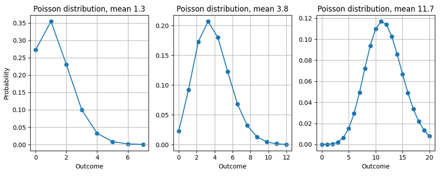
See here what probability distribution we implicitly assert when we predict 1.3, 3.8 or 11.7:
Back to evaluating Absolute Error: How can we subtract a function from a number? Subtracting 7 sold items from a probability distribution makes no sense. We need to summarize the predicted probability distribution by a single number to make a comparison possible. This summary number is called the point estimator, which can then be subtracted from the observed actual value to yield the error.
Probability distributions can be summarized in many ways: The mean is the most immediate, but distributions can also be summarized by their most probable outcome (their mode), by the outcome that divides the probability distribution into two equal halves (their median), or by other prescriptions.
In that zoo of point estimators, some feel more natural than others – can we just choose the summary that we like best? No, the correct point estimator is fixed by the chosen evaluation metric. In other words: You may choose which error metric evaluates my forecast (MAE, MAPE, MSE …), but then I choose how to summarize the forecast for that evaluation. My point estimator for winning at MAE will be different from the one for winning at MSE, let alone MAPE. This choice may sound arbitrary, maybe even dishonest to you, but it reflects the immense expressive power of probabilistic forecasts: They contain much more information than just a single “best guess”. Depending on how they are evaluated, how “best” is actually defined by the error metric, the value that wins for a given evaluation method is chosen accordingly. In other words: The ask “Give me your best forecast” is meaningless as long as it is not clear how “best” is defined. A single probabilistic forecast can produce many different point estimators, or “best guesses,” depending on how the forecast is evaluated.
For Squared Error (SE), the point estimator is the mean of the distribution. For Absolute Percentage Error (APE), the point estimator is a really counter-intuitive functional that I won’t trouble you with, which leads to unexpected paradoxes in MAPE-evaluations.
Absolute Error requires the distribution median, not the mean, and yes, that matters
For AE (Absolute Error), the correct point estimator turns out to be the median. Yes, the median, and not the mean, and no, we can’t just use the mean instead. Let me explain why only the median can be optimal for AE. Let’s take one forecast, that is, one distribution, and let it be the Poisson-distribution with mean 3.8 and median 4. How many items do you stock up when given this forecast? The result is necessarily an integer, it can’t be 3.8. To find the right stock amount, let’s choose the estimate such that the AE that we find on average when observing outcomes from that distribution is as small as possible.
We search for the right point estimator that condenses this entire distribution into a single number, the best stock amount operationally. In this figure, I try out three different estimates (3, 4, 5):
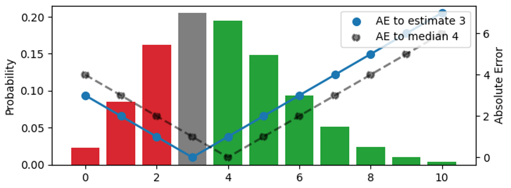
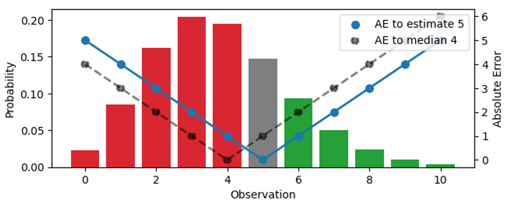
The probability distribution, visualized by the bars (left scale), is the same in the three panels. The upper panel visualizes the estimate 3, in the middle one, the estimate is 4, in the lower one, it’s 5. The AE between the estimate and the outcomes is shown by the blue dots, connected by the solid line (right scale), the AE with respect to the median 4 is shown by black dots, connected by a dashed line. For example, when the estimate is 3 (upper panel), the error for the outcome 3 vanishes, and the blue solid line hits 0. If the observation is 4 or 2, the error is 1.
The color of the bars indicates whether a predicted outcome contributes to the absolute error because it’s smaller (red) or larger (green) than the estimate, the bar height is the probability that it occurs. When an outcome matches the estimate, it contributes zero to the error and is shown in grey. By shifting the estimate up by one unit, we move down by one panel, and all observations under red bars and under the grey bar contribute to one more unit of error for the new, shifted estimate: For the previous estimate 3, the outcome 2 had error 1, but for estimate 4, the same outcome has error 2. On the other hand, all observations that had green bars now contribute to one less unit of error after the shift: For the estimate 3, the outcome 5 had error 2, for the estimate 4, the error decreases to 1.
Let’s summarize what happens when the estimate is increased by one unit: The expected value of AE under the distribution increases for those outcomes that are smaller than or equal the estimate (we over-forecast them even more than we did) and decreases for those that are larger than the estimate (we under-forecast them less). The increase is proportional to the total area of the red and grey bars, the decrease is proportional to the area of the green bars.
In full analogy, when decreasing the estimate by one unit, observations under green bars or under the grey bar contribute to one more unit of error each, and all observations in the red bars contribute to one less unit of error.
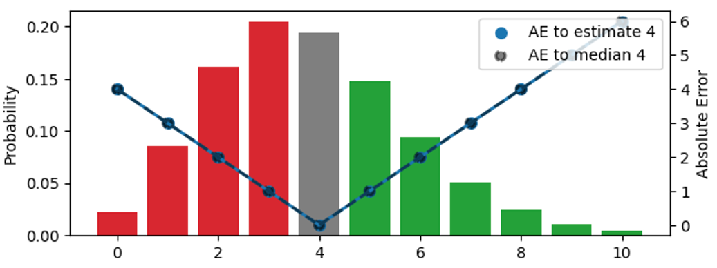
For a given distribution, shifting the estimate up and down by one increases or decreases the resulting expected absolute error, and we can search the right point estimate by looking for the minimum. You might have already devised this rule of thumb: If, for the current estimate, most outcomes are under-predictions, decrease the estimate; if most outcomes are over-predictions, increase it. Only when the difference between the probability masses related to over- and under-predictions (the difference between the total areas of “red” and “green” bars) is smaller than the grey bar, one cannot improve the error any further. This is the case in the middle panel: The estimate is such that the probability masses below and above it nearly coincide, such that moving in either direction would increase the total error. This estimate matches the median: When you are given a probability distribution, the point estimator that minimizes absolute error will be higher or lower than the outcomes in half of the cases.
I believe it’s worth stressing this point, because it often remains unaccounted: When 7.3 is the best estimate for the mean of a distribution, the correct way to evaluate the absolute error against an observation of, say, 9, is not to subtract 7.3 from 9, but to subtract the median of that distribution (which is 7 for the Poisson distribution), from 9. Operationally, 7 is precisely the number of items that you would stock up, given a prediction of 7.3. Surprisingly, it does not help you to have a precise estimate of the mean value for stock decisions, it does not matter whether the forecast is 7.1 or 7.3: You need to decide for an integer. However, when aggregating forecasts on a higher level for planning, the distinction between 7.1 and 7.3 becomes important.
This distinction between mean and median may seem to you like splitting hairs: After all, the value that divides the probability in two equal halves and the mean of that distribution seem very similar, and they are close for most benevolent distributions (such as the Poisson distribution that is pertinent for retail). However, two distributions can have the same mean, but different medians; two other distributions might coincide in median but differ in their mean. Just using the mean and median as synonyms would prevent you from really finding the best forecast.
The unexpected shortcomings of Mean Absolute Error We now know to evaluate Absolute Error for probabilistic forecasts: We summarize the distribution by the point estimator median (the number of items that we would stock up), we subtract that median from the observed outcome, and take the absolute value. I’ve tried to visualize this in the following plot:
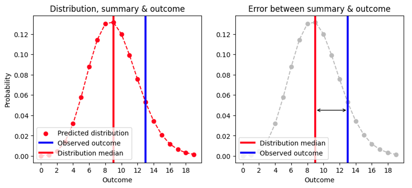
Since the median is always an integer, two quite different distributions can yield the same Absolute Error. For example, the AE for a Poisson-forecast of 8.7 (median=9) and for a Poisson-forecast of 9.6 (median=9) are the same, even though the forecasts are clearly different, as we see in this figure:
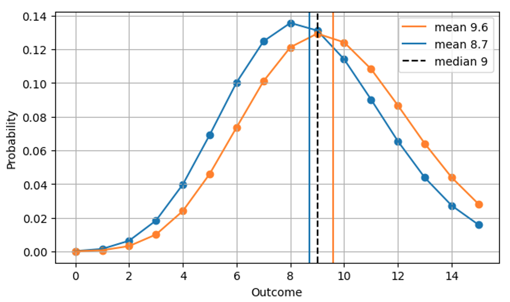
This makes sense operationally: In both cases, the right thing to do is to have 9 items on stock on a given day. Consequently, a more realistic version of the very first figure, AE as a function of the prediction, is the following.
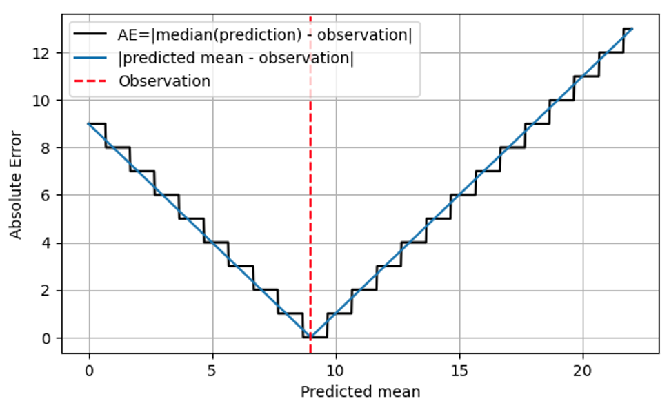
AE is computed using the median of the prediction (black line), and only assumes integer values. I’m being a bit more specific on what the x-axis means: It’s not just “prediction,” but the predicted mean.
This stairway shape implies that AE is coarse-grained and imprecise: We can, by eye, distinguish the distributions with mean 8.7 and 9.6, but AE can’t! MAE alone won’t help you improving the precision of a forecast beyond a certain threshold, which is quite dramatic for slowly moving items: The relative difference between 1.7 and 2.6 amounts to 53%, while the AE of a forecast of 1.7 and that of a forecast of 2.6 are the same! That coarse-grained behavior is coming with nasty jumps, discontinuities at the values at which the median of the distribution jumps from one integer value to the next. Operationally, there is no difference in predicting 1.7 or 2.6 for a given day, location and item: The right amount to stock up is 2. Forecasts are, however, also used on higher aggregation levels for planning. On such high level, one does indeed notice the difference between 1.7 and 2.6: For the next 100 days, it makes a huge difference whether one orders 170 or 260 items at the supplier.
When the predicted mean is below about 0.69 per prediction time period (a slow-seller), the prediction that gives you the best Absolute Error is 0. Quite dramatically, we have the same Absolute Error for a forecast of 0.6, of 0.06 and 0.006, even though we went through two orders of magnitude! The prediction 0 is quite useless in supply chain, as you enter the vicious circle of perfect 0-forecasts: You stock up 0, you sell 0, and your previous forecasted 0 has been self-fulfillingly correct.